|
Multilevel optimization in details
Our multilevel procedure
The typical situation while solving a problem of optimizing a complex
engineering system is that the user has several tools of various degree
of fidelity to perform the analysis. These tools differ in their level
of complexity of modeling the actual physical phenomena and in their level
of numerical accuracy. The high-fidelity (true) tools could be represented
by detailed non-linear mathematical models of the researched systems or
even by the experimental samples of such systems. However, the use of
such tools in optimization is associated with significant time expenditures.
The low-fidelity (surrogate) models could also be employed in optimization
search, but the reliability of the obtained results can be rather low.
Therefore, the methods based on a combination of various fidelity analysis
tools are widely practiced. Our multilevel optimization procedure is based
upon the adaptive use of analysis tools of various levels of complexity.
The intention is to minimize the use of complicated time-consuming tools
for the analysis.
The basic scheme of multilevel optimization
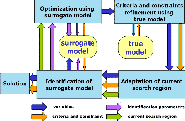
The simplified scheme of work for the multilevel optimization procedure
can be represented as follows.
- Solving the optimization problem using a surrogate model. For this
purpose, the method of indirect optimization based on the self-organization
(IOSO) is used. This method allows finding the single solution for single-objective
optimization or the Pareto-optimal set of solutions for multi-objective
problems.
- For the obtained solution the indicators of efficiency are updated
using the high-fidelity analysis tools.
- The adjustment of a current search region is performed.
- The adjustment of the surrogate model is performed. Depending upon
the particular features of the applied mathematical simulation, the
adjustment procedure can performed using several approaches. One such
approach involves constructing non-linear corrective dependencies. This
includes evaluation of the results obtained with different fidelity
analysis tools. The other possible approach is application of nonlinear
estimation of surrogate model internal parameters.
- Replacement of the surrogate model by the adjusted one and the return
to step I.
The information stored during the search is used to improve the surrogate
model. After the analysis procedure terminates, one can monitor the evaluated
response functions. However, both adjusted model and response functions
are correct not for the entire initial search area but only for a certain
neighborhood of the obtained optimal solution. This ensures purposeful
improvement of approximating properties only in the area of the optimal
solution. Such a procedure noticeably reduces the computation effort of
solving complex optimization problems.
Real-life examples
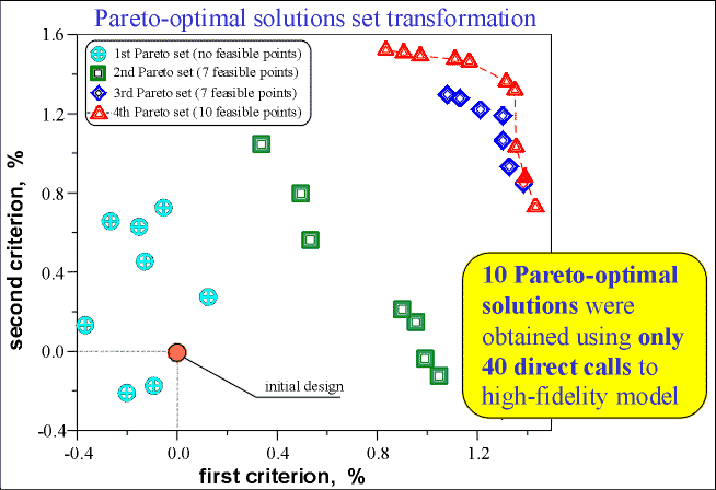
Multilevel Optimization of the Multistage Axial Compressor
Design
Problem features:
| variable parameters: |
inlet an exit angles of 7 blade rows in
3 sections by radius (42 variables) |
| criteria: |
the efficiency at two operating modes (2
criteria) |
| constraints: |
stall margins at two operating modes;
the constraint by criteria computability |
| high-fidelity tool: |
quasi-3D model with viscosity effects simulation |
| low-fidelity tool: |
2D axis symmetric model capable to be
identified |
Result:

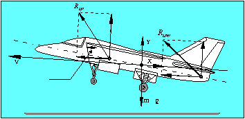
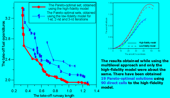
The Multilevel Optimization of Temporal Control Laws
of STOVL Aircraft Power Plant for Short Take-Off
 
variable parameters:
|
the temporal control laws of 10 power plant
independent controllable elements and the aircraft pitch |
| criteria: |
the take-off run length; the take-off fuel
expenditures (2 criteria) |
| constraints: |
the maximum rotors rotation rates and the
turbine inlet temperature; the minimum compressors surge margins;
the flight safety; the criteria computability |
| high-fidelity tool: |
the quasi-steady model of the power plant
in the system of the aircraft. The aircraft was modeled as the material
point |
| low-fidelity tool: |
the same model with simplified procedures
of differential equations numerical integration and the computation
of thermodynamical processes of the power plant |
Result:

Back...
| 
